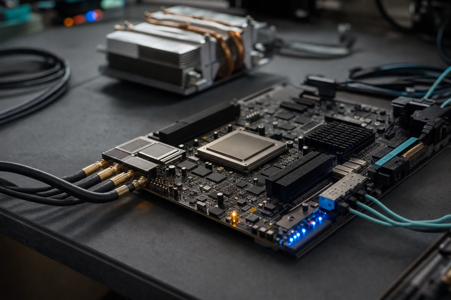
Industry news — On 12 March 2026 CAST released TSN-EP-10G, a 10 Gigabit Time-Sensitive Networking endpoint core that implements IEEE 802.1AS-2020 gPTP, 802.1Qav credit-based shaping and 802.1Qbv time-aware scheduling in hardware, with a claimed synchronisation accuracy better than 10 nanoseconds — a bound no software scheduler running on a general-purpose CPU is asked to guarantee (Design&Reuse, 12 March 2026).
In short: a CPU is the right answer for most data paths, and the FPGA vs CPU question is really a question about worst cases — fabric wins when the specification is written as a bound on latency, jitter or buffering that software cannot structurally guarantee.
The number worth noticing in that announcement is not 10 Gigabits. It is 10 nanoseconds. Synchronisation held to that bound is not a feature you bolt onto a network stack; it is a consequence of where the timestamping and the scheduling happen. Put them in software on a general-purpose processor and the figure stops being a bound and becomes an average with a tail. Put them in fabric and the figure is a count of clock cycles that you can read off the design. Determinism, in other words, is a structural property rather than an optimisation — and that single observation is the whole of the FPGA vs CPU question. This article tries to draw the line honestly: the CPU is the right answer for most data paths, and the useful work is in naming precisely the conditions under which it stops being.
- The short answer
- CPU and FPGA: two ways to spend the same transistors
- Latency and jitter, not throughput, are the real argument
- Where the CPU wins, which is most of the time
- Where the FPGA wins
- The hybrid answer: a CPU next to the fabric
- The honest cost side
- A decision framework: six questions
- Where this stops applying
- Frequently asked questions
The short answer
A CPU is a small number of extremely fast execution units that the whole of your
program takes turns using; an FPGA is your data path laid out in silicon, with every stage of it
running on every clock edge. That difference does not make an FPGA faster in general — a
modern server processor has aggregate throughput a mid-range fabric cannot approach on
general-purpose work, and it will out-run hand-written RTL on anything with irregular control flow
or heavy floating-point maths. What the FPGA is, and the CPU is not, is bounded. If your
requirement is written as a worst case rather than an average — a frame that must not be
dropped at line rate, a control loop that must respond within a fixed number of microseconds, an
ingest stream with a hard limit on how much you are allowed to buffer — then the FPGA is the
structure that can guarantee it and the CPU is the structure that cannot. Everything below follows
from that one asymmetry.
CPU and FPGA: two ways to spend the same transistors
A CPU and an FPGA are two answers to the same question: given a fixed budget of silicon, how do
you make it compute arbitrary things? The answers are opposites, and almost every practical
difference between the two devices is downstream of the choice.
The CPU: reuse in time
A processor spends its transistors on a handful of very wide, very fast, very deeply optimised
execution units and then shares them out over time. Your algorithm is decomposed into a fixed
instruction set, and those instructions stream through the same adders and multipliers one after
another. This is temporal parallelism: apparent concurrency obtained by switching a small
amount of hardware between many tasks quickly, whether that switching is done by an out-of-order
issue window, by simultaneous multithreading, or by an operating-system scheduler.
Everything a modern CPU is famous for exists to keep those few units fed. Caches hide the fact
that DRAM is hundreds of cycles away; branch prediction and speculation hide the fact that the next
instruction is not known yet; an out-of-order engine reorders work around stalls. Every one of those
mechanisms raises average performance by making the time an individual operation takes depend on
history — on what ran before it, on what is resident in the cache, on which core the scheduler
picked. And between your code and the wire sit a compiler, a runtime, a driver, an interrupt
controller and a kernel scheduler, each entitled to interpose.
The FPGA: reuse in space
An FPGA spends its transistors on a large field of small, slow, configurable elements —
lookup tables, flip-flops, block RAMs, DSP slices — and lets you wire them into the shape of
your algorithm. Nothing is reused over time unless you choose to reuse it. If your data path has
eight filter taps, you can instantiate eight multipliers and compute all eight every clock. This is
spatial parallelism: concurrency obtained by having physically separate hardware for
physically separate work.
The technique that turns spatial layout into throughput is pipelining — cutting a
long combinational path into stages separated by registers, so that a new input can be accepted
before the previous one has finished. The figure that matters is then not how long one item takes
but how often you can start a new one, the initiation interval. A data path with an
initiation interval of one accepts a new sample on every single clock edge, forever, regardless of
what the previous samples were. Its total delay is the pipeline depth, which is a constant you can
count in the schematic. There is no scheduler, no cache, no speculation and no history.
Individual FPGA logic is much slower than a CPU core: a fabric design typically closes timing
somewhere in the low hundreds of megahertz, and the LDS I2C master core states its own ceiling in
exactly those terms — “FPGA speed grade operating frequency dependant : system clock up
to 180 MHz”. A processor running above 3 GHz is an order of magnitude ahead per
operation. The fabric compensates by doing hundreds of operations per clock instead of a handful,
and by never being interrupted. Whether that trade is worth making is the rest of this article.
Latency and jitter, not throughput, are the real argument
Throughput is the wrong axis on which to argue this, and using it is how FPGA marketing loses
credibility with people who have actually measured a server. A modern multi-socket CPU has enormous
aggregate bandwidth and enough cores to saturate several network interfaces at once. If your
requirement is “process this many gigabytes per hour”, buying processors is almost
always cheaper than designing hardware.
What a general-purpose CPU cannot offer is a bounded worst case. Determinism here
means that the same input always produces its output after the same number of clock cycles, and
jitter means the spread between the fastest and slowest response the system will ever
produce. On a fabric data path, jitter is zero by construction. On a processor, every mechanism
listed in the previous section contributes to it:
- Interrupt latency. The time between a device asserting an interrupt and your
handler executing is not a constant. It depends on what the core was doing, on whether interrupts
were masked in a critical section, and on how many other handlers are queued ahead of yours. - Cache and TLB misses. A load that hits L1 costs a few cycles; the same load
missing to DRAM costs hundreds. Which one you get depends on what else has run recently, including
code that is not yours. - NUMA and memory placement. On a multi-socket machine, whether a buffer is local
to the core touching it changes access cost materially, and the placement is decided by an allocator
you do not directly control. - Kernel preemption and scheduling. Even a real-time kernel makes latency
bounded in practice rather than bounded by construction, and the bound is measured
empirically per platform, per kernel version and per workload. - Frequency and thermal management. Clock throttling, power states and turbo
residency all change instruction timing between one run and the next.
The consequence is that a CPU data path has a mean latency that is genuinely excellent and a tail
that is genuinely unbounded. Designs are not killed by the mean. They are killed by the p99.99
— the one response in ten thousand that arrives late, drops the frame, misses the control
deadline or overruns the capture buffer. Averaged over an hour a system can look perfect and still
be unshippable, because the specification says “shall not drop a frame” and not
“shall rarely drop a frame”. When you find yourself buying headroom — a faster
processor, more cores, a bigger buffer — purely to push a tail below a threshold, that is the
signal that the requirement is a hardware requirement.
Where the CPU wins, which is most of the time
For most data paths the CPU is the right answer, and saying so plainly is the only way the rest
of this page is worth reading. Software wins whenever any of the following is true, and in practice
at least one of them usually is.
- The control flow is irregular. Parsing, tree walking, branchy business logic and
anything data-dependent maps badly onto a fixed pipeline. A branch predictor with a good hit rate is
a remarkable piece of engineering, and there is no fabric equivalent. - The maths is floating-point and a good library exists. Decades of tuned BLAS,
FFT and codec implementations run on hardware designed to execute them. Re-deriving that in RTL is a
research project, not a design task. - The requirement is a millisecond, not a microsecond. If a 10 ms response is
acceptable, an ordinary Linux userspace process will meet it with margin to spare and you should
stop the analysis there. - The algorithm is still moving. Rapid iteration is where software is unbeatable.
Changing a constant is a recompile measured in seconds. - You need to hire next month. The pool of competent C, C++, Rust and Python
engineers is orders of magnitude larger than the pool of engineers who can close timing on a
high-speed interface. This is a real engineering constraint, not a soft one. - The work is bursty and the average load is low. A processor that is idle 95% of
the time costs you nothing extra; fabric you instantiated is occupied whether or not data arrives.
Notice that none of these is about speed. The CPU’s advantages are flexibility, ecosystem, cost
of change and cost of people. Those are the advantages that decide most projects, which is exactly
why an FPGA has to be justified by a requirement that software structurally cannot meet.
Where the FPGA wins
The FPGA wins where the requirement is stated as a bound and the I/O will not wait. Five patterns
recur, and each of them shows up in the storage, avionics and networking work an IP vendor sees.
Line-rate protocol handling that must not drop a frame
At 10 Gbps, a minimum-size Ethernet frame occupies 64 bytes of frame plus 8 bytes
of preamble and start-of-frame delimiter, followed by an inter-frame gap of 96 bits —
12 bytes. That is 84 bytes, or 672 bits, on the wire per frame: 67.2 ns at the
line rate, which is a shade under 14.9 million frames every second. Those parameters come from IEEE
802.3; the arithmetic is just division. A classifier that must inspect every frame therefore has a
per-frame budget of tens of nanoseconds with no option to fall behind, because the wire does not
apply back-pressure. In fabric that is an ordinary pipeline. In software it is a specialist
discipline of kernel bypass, busy-polling and pinned cores, and the tail is still there. This is the
world a 10G Ethernet MAC IP
core lives in, and it is why the LDS MAC is documented as “designed to be connected to a
PCS/PMA IP with only one clock domain” — one clock, no domain crossing, no queueing
surprise.
Sustained ingest with a hard bound on buffering
A recorder is the purest form of the argument. Data arrives at a rate set by the outside world,
and the only two outcomes are that you write all of it or you lose some of it. If the write path can
stall unpredictably, the buffer must be sized for the worst stall you have ever observed rather than
for the one you can prove. LDS published a single figure here, in a 2019 news item: roughly
500 MBytes per second sustained over one 6 Gbps SATA link. The architecture behind that
— a SATA III recorder
built as fabric, and its
NVMe host recorder
counterpart with 512 bytes or 4096 bytes sector sizes and up to 16 independent I/O queues
— exists so that the ingest path contains no software at all and the buffer can be sized from
the design rather than from a histogram.
Hard real-time control and sensor front ends
A control loop with a deadline expressed in microseconds, an ADC that must be sampled on a fixed
phase, a motor commutation that must not glitch: these are cases where a late answer is a wrong
answer. Fabric gives the loop a fixed number of clock cycles from sample to actuation, and the
number does not change when someone else logs into the machine.
Deterministic data buses in avionics
ARINC 429 is a low-rate bus by modern standards, but the requirement is not rate — it is
that every word of every label is received, timestamped and filtered without exception, on equipment
that has to be certifiable. The
LDS ARINC 429 IP core handles
independent receivers and transmitters with their own FIFOs, multi-label filtering and per-direction
interrupts, and its product page states support for “all ARINC 429 Data Rate Transfer and up
to 2.5 Mbit/s”. Doing label filtering in fabric means the CPU is never woken for traffic it
does not want, and it means the evidence trail for certification covers a bounded state machine
rather than an operating system. The same page notes that DO-254 design, verification and
traceability documentation is available on request, which is the other half of why this work sits in
hardware.
I/O counts a processor package cannot physically provide
Sometimes the argument is not timing at all. If you need forty independent serial channels, a
dozen LVDS sensor lanes and a handful of legacy parallel buses on one board, no processor package
exposes that many pins with that mix of standards. An FPGA does, and the glue logic that would
otherwise be a bag of discrete components becomes a set of soft cores — I2C, SPI and UART
macros delivered as VHDL source — inside one device. That is a packaging and obsolescence
argument rather than a performance one, and it is a perfectly good reason on its own. The related
question of where a microcontroller stops being enough is covered separately in
FPGA vs microcontroller for high-throughput
I/O.
The hybrid answer: a CPU next to the fabric
For most real systems the answer is neither device but both, and the modern way to get both is an
SoC FPGA: hard processor cores fabricated in the same die as the programmable fabric, sharing memory
and an on-chip interconnect. The split that works is almost always the same one. The data path
— the part with the deadline — is fabric. The control plane is Linux on the hard cores:
configuration, the management interface, logging, the web UI, firmware update, the parts of the
system that change often and have no deadline. All three FPGA vendors ship families built for
exactly this, and the processor complexes differ enough to matter.
| Vendor | SoC family | Hard processor complex |
|---|---|---|
| AMD | Zynq 7000 / 7000S SoC | Dual-core Arm Cortex-A9 MPCore, or a single-core Cortex-A9 on the 7000S entry devices, beside 28 nm Artix 7 or Kintex 7 class fabric |
| AMD | Zynq UltraScale+ MPSoC | Application unit of “Quad-core Arm Cortex-A53 MPCore” on EG and EV devices (dual-core on CG), plus a separate real-time unit of “Dual-core Arm Cortex-R5F MPCore” |
| AMD | Versal adaptive SoC (Prime, AI Core) | Dual-core Arm Cortex-A72 application unit with ECC-protected caches, plus a dual-core Arm Cortex-R5F real-time unit, connected by a hardened network-on-chip |
| Altera | Agilex 7 SoC, Stratix 10 SoC | Quad-core Arm Cortex-A53 hard processor system alongside the high-end fabric and transceivers |
| Altera | Arria 10 SoC, Cyclone V SoC | Dual-core Arm Cortex-A9 hard processor system, the mid-range and low-cost entry points |
| Microchip | PolarFire SoC | A 64-bit RISC-V complex: four Linux-capable RV64GC application cores plus a monitor core, with an L2 memory subsystem that can be partitioned as a deterministic scratchpad |
| Microchip | SmartFusion2 | A hard Arm Cortex-M3 microcontroller subsystem — a control processor rather than a Linux host, on flash-based fabric |
Two details in that table are worth pulling out. The first is the presence of a separate
real-time processing unit on the AMD parts: the Cortex-R5F cores exist precisely because the
application cores running Linux are not the place for a deadline, so the vendors put a third tier
between fabric and Linux. The second is that Microchip’s route to the same problem is a RISC-V
complex with a memory subsystem that can be locked down for predictable access, which matters when
the control plane itself has real-time obligations.
The split also changes what an FPGA project costs: you write RTL only for the part with a
deadline, and the configuration and management code stays in a language your team already writes.
Getting the boundary right — which registers the processor sees, what the interconnect looks
like, who owns the buffer — is then most of the architecture work.
The honest cost side
The real cost of an FPGA data path is not the device, and quoting device prices is how these
comparisons go wrong. The cost is in the development model, and it differs from software in ways
that compound.
- The edit-test loop is minutes to hours, not seconds. A change that is a
recompile in C is a synthesis, place-and-route and timing-analysis run on an FPGA. On a large device
that is a coffee break at best and an overnight job at worst, and it happens on every iteration. - Timing closure is a distinct discipline. Meeting the frequency you designed for
is not automatic; it is constraint writing, floorplanning, pipelining and retiming, and it gets
harder as the device fills. High-speed interfaces are where it bites hardest. - Verification is most of the work. There is no debugger you can attach to a
running pipeline in the way you attach to a process. You verify in simulation with testbenches you
also have to write, and instrumenting hardware costs fabric. - Tool licences and build infrastructure cost money and administration, and the
premium editions needed for the largest devices are not free. - The hiring pool is small. Digital design engineers who can take a protocol from
specification to closed timing are scarce, and that scarcity is permanent enough to be a planning
assumption rather than a temporary market condition.
This is the strongest argument for buying rather than building the standard parts of the data
path. A protocol engine delivered as verified VHDL or Verilog source, with drivers in C, removes the
part of the schedule that is pure specification compliance and leaves your team the part that is
actually your product. The trade-off between reprogrammable fabric and a fixed-function device,
including the volume at which the arithmetic changes, is a different decision that belongs to
FPGA vs ASIC and why IP reuse
matters; and if you are still at the stage of deciding what a soft core actually is, start with
soft IP vs hard IP.
A decision framework: six questions
Six questions are usually enough to settle the argument, and they are ordered so that the first
“yes” that matters ends the discussion.
1. Is your requirement written as a worst case?
If the specification says “shall respond within” or “shall not drop”, and
a single violation is a failure — FPGA. If it says “shall average”
or the tail is merely undesirable — CPU.
2. Is the deadline shorter than roughly a millisecond?
Below tens of microseconds, and certainly below one, software is fighting its own architecture
— FPGA. At a millisecond or more, an ordinary process meets it —
CPU.
3. Does data arrive whether or not you are ready?
If the source cannot be back-pressured — a wire, a sensor, a radio, a bus — and the
buffer must be bounded, then FPGA. If you control the producer, or a queue can
absorb a hiccup, then CPU.
4. Is the processing structure fixed?
Filters, CRCs, framing, ciphers, correlators, protocol state machines all map cleanly onto a
pipeline — FPGA. Branchy, data-dependent, library-heavy or floating-point work
— CPU.
5. Do you need I/O the processor package cannot give you?
Many channels, unusual standards, exact pin timing, or a long production life that has to survive
component obsolescence — FPGA. Standard interfaces in ordinary quantities
— CPU.
6. How often will this change after it ships?
If the algorithm is still being discovered, or the field expects frequent updates to the logic
itself, that argues for CPU — or for putting only the settled part in fabric
and leaving the rest in software on the same SoC. If the function is a standard that will outlive the
product, FPGA.
Read the answers together rather than counting them. In practice a clear yes to question one or
question three usually decides the data path on its own, and questions four to six then decide how
much of the system follows it into hardware. If you are working through this for the first time, the
companion piece what an FPGA
actually is covers the device-level vocabulary this framework assumes.
Tell us the protocol, the target device and the deadline you have to meet, and we will say plainly whether the data path belongs in fabric, in software, or split across an SoC FPGA.
Where this stops applying
This is a comparison of two structures, not a benchmark, and it has firm boundaries:
- No performance ratios are claimed here. This article contains no speed-up
factor, because a meaningful one exists only for a named workload on a named device with a named
compiler and a named configuration. Any figure quoted without all four is marketing. - The only measured throughput cited is the one LDS has published: roughly
500 MBytes per second sustained on a single 6 Gbps SATA link, from a 2019 news item.
Resource utilisation, latency and power figures for LDS cores are not published; treat any number
you have not received in writing for your device and configuration as unknown. - Real-time operating systems narrow the gap and do not close it. A properly
configured RT kernel with isolated cores gets latency bounds that are excellent and empirically
established. They remain empirical: measured on a platform, not derived from the design. - GPUs and dedicated accelerators are outside this comparison. For dense regular
maths on large batches they beat both devices discussed here, and they lose on latency bounds and
I/O for the same reasons a CPU does. - Whether to use fabric at all versus a fixed-function device is a separate
question of volume, non-recurring engineering and product lifetime, argued elsewhere and not
re-argued here.
In summary
The FPGA vs CPU comparison is decided by the shape of the requirement, not by a
performance table. A CPU executes a fixed instruction set over time, with caches, speculation and a
scheduler standing between your code and the wire, and it delivers an excellent average with a tail
nobody can bound from first principles. An FPGA lays the data path out in space and runs all of it
on every clock, so its latency is a pipeline depth you can count and its jitter is zero. Neither
property makes one device better; they make them suited to different sentences in a specification.
When the sentence contains the word “shall” and a deadline, that is the fabric’s
sentence.
In practice the answer for most systems is an SoC FPGA and a clean split: the deadline in
hardware, the control plane in Linux on the hard cores that AMD, Altera and Microchip put beside the
fabric. That keeps the expensive part of hardware development confined to the part that needs it,
and it is why the data paths worth moving into fabric — continuous storage recording,
line-rate frame classification, avionics label filtering — tend to be bought as verified
source-code IP rather than rewritten each time.
Frequently asked questions
Is an FPGA always faster than a CPU?
No, and the claim does not survive contact with a benchmark. A modern processor core runs an order of magnitude faster per operation than fabric logic and has decades of tuned libraries behind it, so on irregular or floating-point work it wins outright. What an FPGA offers is a different property: every stage of the data path executes on every clock, so the response time is a fixed pipeline depth rather than an average with a tail. Choose it for bounds, not for speed.
What latency can an FPGA actually guarantee?
A number of clock cycles, which you convert to time using the clock period you closed timing at. That is the useful answer, because it is derived from the design rather than measured on a platform: a pipeline of forty stages at 200 MHz responds in 200 ns every single time. The end-to-end figure then depends on what sits either side of the fabric — transceivers, external memory, the sensor itself. Ask a vendor for the figure against your device and configuration, and treat unqualified numbers as unknown.
Why does jitter matter more than average latency?
Because specifications are written as bounds and failures happen in the tail. A system with a 5 microsecond mean and an occasional 900 microsecond outlier will pass every casual measurement and still drop a frame or miss a control deadline once every few hours. When the acceptance criterion is that a violation must never occur, the distribution’s worst case is the only figure with any standing, and averages actively mislead the people reading the test report.
Can a real-time operating system solve the determinism problem?
It narrows the gap considerably and does not close it. An RT kernel with isolated cores, pinned interrupts, disabled power management and locked memory can reach latency bounds that are excellent for most industrial work. But those bounds are established empirically for one platform, one kernel version and one workload, and they must be re-established when any of the three changes. A fabric pipeline’s bound is a property of the design and does not move.
How much longer does an FPGA data path take to develop?
Longer than software, and the honest answer depends on how much of the path you write yourself. The costs that compound are the build loop — synthesis, place and route, timing analysis, measured in minutes to hours rather than seconds — and verification, which is most of the effort and has no runtime debugger. Licensing verified protocol IP as VHDL or Verilog source removes the specification-compliance part of the schedule and leaves the part that is actually your product.
Should the control plane run on the FPGA too?
Usually not. The productive split on an SoC FPGA is to put the deadline in fabric and everything else on the hard processors: configuration, management interfaces, logging, firmware update. AMD offers Arm Cortex-A53 or Cortex-A72 application cores with separate Cortex-R5F real-time cores, Altera an Arm Cortex-A53 or Cortex-A9 hard processor system, Microchip a RISC-V complex on PolarFire SoC. Writing RTL for work with no deadline spends the expensive resource on the cheap problem.
- IEEE 802.3 Ethernet Working Group — IEEE 802.3 Ethernet Standard: the frame, preamble and inter-frame gap parameters behind the minimum-size frame arithmetic quoted in this article.
- AMD — Zynq UltraScale+ MPSoC product page: the quad-core Arm Cortex-A53 application unit and dual-core Cortex-R5F real-time unit quoted in the SoC table.
- AMD — Versal Prime series product page: the dual-core Arm Cortex-A72 application unit and dual-core Cortex-R5F real-time unit of the Versal adaptive SoC.
- AMD — Zynq 7000 SoC product page: the single-core and dual-core Arm Cortex-A9 processing systems of the Zynq 7000 family.
- Altera — Agilex 7 FPGAs and SoCs: the Agilex 7 SoC hard processor system referenced in the SoC table.
- Altera — FPGA and SoC FPGA product families: the Stratix, Arria and Cyclone SoC families and their Arm hard processor systems.
- Microchip Technology — PolarFire SoC FPGAs: the RISC-V application and monitor cores and the L2 memory subsystem cited for PolarFire SoC.
- Logic Design Solutions — ARINC 429 IP (M429GEN) product page: the multi-label filtering, independent Rx/Tx FIFOs and the quoted data-rate support up to 2.5 Mbit/s.
- Design&Reuse — CAST debuts TSN-EP-10G IP for time-sensitive networking Ethernet designs, 12 March 2026: the March 2026 announcement cited in the opening, including the sub-10 nanosecond synchronisation claim.