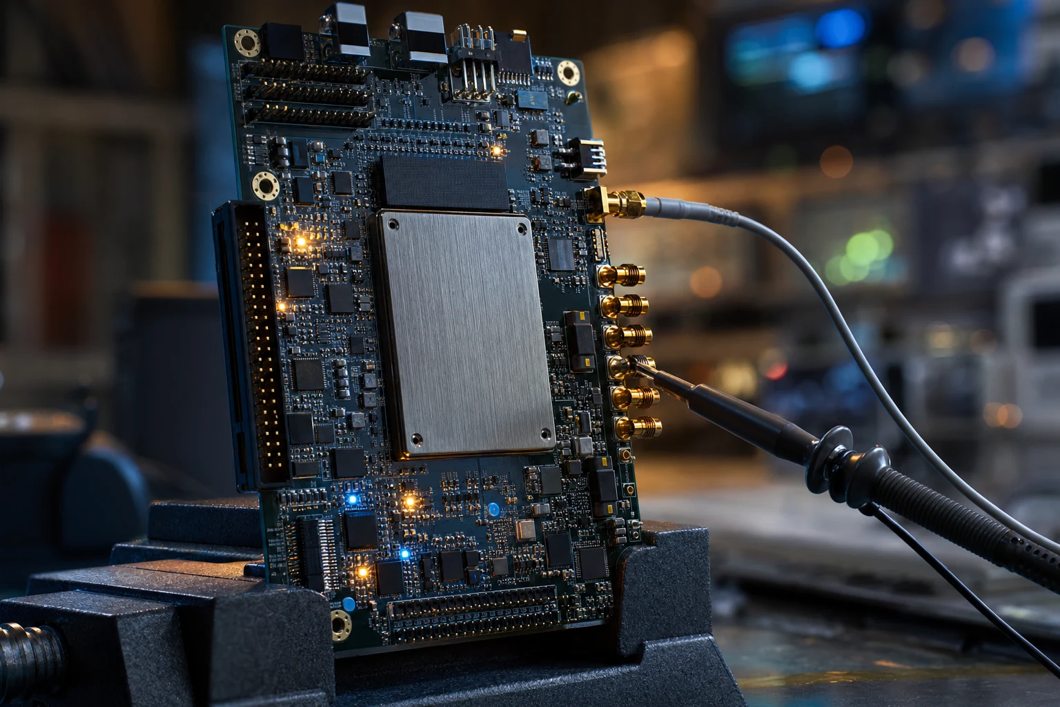
Industry news — Altera shipped Quartus Prime Pro Edition 26.1 on 6 April 2026 and put figures on the two things an FPGA schedule is actually made of: “Agilex 7 designs experience over a 9% reduction in runtime, while Agilex 5 designs see a 5.5% reduction in runtime, all with no increase in memory usage”, with restricted Fmax up 0.6% on Agilex 7 and 3.3% on Agilex 5. Compile time and achievable clock rate are the currency of this flow, and a point release moves both (Altera Community, 6 April 2026).
In short: The FPGA design flow runs in eight stages — specification, RTL entry, verification, synthesis, implementation, timing closure, bitstream, bring-up — each of which can reject the one before it, and its verdict depends on the device, the tool version and the constraint set as much as on the source code.
Those two percentages are worth dwelling on, because they describe the whole problem. A tool release did not change one line of anybody’s RTL, and yet it changed how long a build takes and what clock rate the result will hold. That is the defining property of the FPGA design flow: it is a chain of transformations, each of which can reject the work of every stage before it, and the verdict at the end is not a property of the source code alone. Engineers who live in this flow know that instinctively. Programme managers, procurement leads and system architects buying an FPGA subsystem often do not, and it is usually why an FPGA schedule surprises them.
What follows walks the flow end to end in the order it actually runs, says what each stage consumes and produces, and is explicit about which stage rejects what. It is written for the reader who has to plan, budget or buy an FPGA development without being the one writing the Verilog.
- The short answer
- The stages, and what each one can reject
- Specification, design entry and the constraint set
- Synthesis: RTL becomes a netlist of primitives
- Implementation: placement, routing and physical reality
- Timing closure and the bitstream: the last gate
- Where a licensed IP core enters the flow
- Where this stops applying
- Frequently asked questions
The short answer
The FPGA design flow is the fixed sequence that turns a written
specification into a configuration file a device can load, and it runs in eight stages:
specification, design entry in RTL, functional
verification, synthesis, implementation (placement and routing), static timing analysis and
timing closure, bitstream generation, and hardware bring-up. Each stage consumes the output of
the last and can reject it. The two stages that dominate a real schedule are not the ones
newcomers expect: verification, which routinely takes more calendar time than design entry, and
timing closure, which is where a functionally correct design discovers it cannot run fast enough
on the device that was chosen for it.
Two properties of the flow explain most of the surprises. First, it is iterative, not
linear: a failure at implementation sends you back to RTL, and a failure at bring-up can
send you back to the specification. Second, the result is not reproducible across a change of
device, speed grade, tool version or constraint file. That is not a defect of the tools. It is
what it means to map a design onto physical silicon whose delays are extracted, characterised and
re-characterised over time.
The stages, and what each one can reject
Each stage of the flow is a gate with its own failure mode, and knowing which
gate rejects what is the fastest way to read an FPGA schedule. A functional bug found in
simulation costs hours; the same bug found at bring-up costs a board spin. The table below is the
version of the flow worth carrying in your head.
| Stage | Consumes | Produces | Rejects |
|---|---|---|---|
| Specification | System requirements, interface standards | Micro-architecture, block diagram, budgets | Requirements no device can meet |
| Design entry (RTL) | Micro-architecture | Verilog, VHDL or SystemVerilog source | Non-synthesisable constructs |
| Functional verification | RTL plus a testbench | Coverage and regression results | Behaviour that does not match the specification |
| Synthesis | RTL, constraints, device target | Netlist of device primitives | Designs that do not fit, and inferred latches |
| Implementation | Netlist, constraints, pin assignment | Placed and routed design | Congestion, unroutable designs, I/O rule violations |
| Static timing analysis | Routed design, timing constraints | Slack reports per path | Any path with negative slack |
| Bitstream generation | Fully closed routed design | Configuration file for the device | Designs with unresolved rule-check violations |
| Bring-up | Bitstream, board, instruments | A working system | Everything the previous stages could not model |
Read the right-hand column as a cost ladder. The stages are ordered so that cheap gates come
first, and the discipline of the flow consists of refusing to skip a cheap gate in order to reach
an expensive one sooner. Teams that run implementation before their regression suite passes are
not moving faster; they are buying the same information at ten times the price.
Specification, design entry and the constraint set
Design entry consists of writing synthesisable RTL in Verilog, VHDL or
SystemVerilog, and the constraint set that accompanies it is a first-class deliverable rather than
an afterthought. RTL describes hardware as registers and the combinational logic
between them, and the language is standardised: SystemVerilog is defined by IEEE 1800, whose
current revision is IEEE 1800-2023. The critical discipline is that RTL is not a program. Every
line describes structure that will exist simultaneously in silicon, which is why the same engineer
who writes correct C can write RTL that simulates perfectly and synthesises into something
unusable.
The constraint set is the other half of the input, and it is the half most often
underestimated. Constraints tell the tools what the hardware actually is: which clocks exist and
at what period, what the delay is on signals entering and leaving the device, which paths are
genuinely asynchronous and can be excluded from analysis, and which paths are allowed more than
one clock cycle. AMD’s constraint reference, UG903, covers clock definition, input and output
delay, and the false-path and multicycle exceptions. A design with no constraint file will happily
report that it meets timing, because a tool that has not been told about a clock will not analyse
paths on it. That is the single most common way an inexperienced flow produces a green report and
a dead board.
Three practical consequences follow for anyone planning this work:
- Interface standards fix the arithmetic before any code is written. A storage
data path inherits its clock and datapath width from the standard it implements. The link rates
published by NVM Express and PCI-SIG are what determine whether the fabric sees 128-bit words at
one frequency or 256-bit words at another; it is not a preference. - The pin assignment is a hardware decision taken during design. Which
transceiver bank a link lands in constrains the floorplan permanently, and it is fixed on the
schematic long before anyone runs implementation. - Constraints are reviewed like code. They are reviewed, versioned and
regression-tested, because an over-broad false path silently deletes real analysis.
Synthesis: RTL becomes a netlist of primitives
Synthesis is the stage that translates RTL into a netlist of the specific
primitives a target device physically contains — lookup tables, flip-flops, block RAMs, DSP
blocks and hard IP instances — under the timing constraints supplied with it. It is where
the design first meets the real device, and it is where the first honest resource number appears.
Before synthesis, a resource estimate is arithmetic on a whiteboard; after it, there is a
report.
Two things happen here that regularly surprise people arriving from software. The first is
inference: the tool recognises coding patterns and maps them onto dedicated hardware.
A multiplier written as an ordinary expression becomes a DSP block; an array indexed by a
registered address becomes a block RAM. Write the same function slightly differently and it
becomes hundreds of lookup tables instead, with entirely different timing. The second is that
synthesis optimises across module boundaries, so the hierarchy visible in the source is not
necessarily the hierarchy present in the netlist — which is exactly why analysing a timing
failure means reading the implemented design, not the source.
Synthesis also rejects. A design that does not fit the device is caught here, cheaply, before
hours of placement and routing are spent on it. So are inferred latches, one of the classic RTL
defects: a combinational block that does not assign an output in every branch produces a
level-sensitive element nobody intended and static timing analysis cannot properly bound. Vendors
publish methodology guidance on all of this — the UltraFast Design Methodology Guide, UG949,
is AMD’s reference for its own devices — and the guidance is worth following precisely
because it encodes what the tool’s own optimisers expect to see.
Implementation: placement, routing and physical reality
Implementation takes the netlist and decides where every primitive physically
sits on the die and which wires connect them, and it is the stage where the design stops being an
abstraction. On an FPGA the routing fabric is fixed at manufacture: the tool is not drawing wires,
it is choosing a path through a finite pre-existing network of segments and switches. That
constraint is what makes congestion a real and distinct failure mode, separate from timing.
Placement decides locality, and locality decides delay. Two registers placed near each other on
the die have a short, fast connection between them; the same two registers separated across the
device may not make a 300 MHz period no matter how the logic is written. This is why the
physical arrangement of a device matters when selecting one, and why a wide storage datapath is
usually kept close to the transceiver bank it feeds. Routing then commits those decisions, and the
delays it produces are the ones static timing analysis will judge.
Implementation is also where compile time becomes a schedule item rather than an inconvenience.
Place-and-route on a large design is measured in hours, and an engineer chasing a marginal path
gets a small number of experiments per working day. That is the reason a vendor announcing a
single-digit percentage cut in runtime, as Altera did with Quartus Prime Pro 26.1, is making a
statement about engineering throughput rather than about benchmarks: it is one more attempt per
day per engineer. It is also why the commercial terms of the toolchain now belong in a project
plan. AMD moved Vivado to “a new tiered licensing model starting with the 2026.1
release”, and the published feature matrix places “QoR (RQA, RQS, IDR), Incremental
Compile” outside the entry tier — precisely the convergence aids a team reaches for
when a design misses its target frequency.
Timing closure and the bitstream: the last gate
Timing closure is the state in which every path in the routed design satisfies
its setup and hold requirements in every corner the tool analyses, and it is the last gate before
a bitstream exists. Static timing analysis reaches that verdict exhaustively and
without simulation: it walks every path, adds up the delays the router actually produced, compares
them against the constraint set, and reports slack, the margin by which each path
passes or fails. Negative slack anywhere means no bitstream, and the fixes range from cheap
(retiming, adding a pipeline stage) to expensive (re-architecting the datapath, or changing the
device).
That is deliberately the short version. Closure on a wide, high-rate storage interface is a
discipline of its own — clock domain crossings, floorplanning, pipelining, and a method for
converging rather than thrashing — and it is treated properly in
FPGA timing closure for
high-speed storage interfaces. What matters at the level of this article is the sequencing:
closure comes last, it judges physical results rather than intentions, and a design that reaches
it with no margin has usually made an architectural decision several months earlier that nobody
recorded as a risk.
Bitstream generation is then close to administrative, and bring-up is where the flow finds out
what it could not model: power integrity, signal integrity on the board, and the behaviour of a
real device at the other end of a link. Verification, meanwhile, runs alongside all of it rather
than after it, and the methodology is standardised. The Universal Verification Methodology
maintained by Accellera is the industry framework for constrained-random, coverage-driven
testbenches, built on IEEE 1800 SystemVerilog. Simulation proves the design does what the
specification says. Hardware proves the specification was right.
Where a licensed IP core enters the flow
A licensed IP core enters at design entry and removes work from every stage
downstream of it, which is the whole of its economic argument. A protocol controller — SATA,
NVMe, ARINC 429, a 10G Ethernet MAC — is a block of RTL that has already been written,
already been verified against the standard, and already been closed at frequency on the device
families it targets. The buyer is not acquiring the source alone. They are acquiring the
verification result and the closure result that came with it.
That distinction is worth being precise about, because it is where build-versus-buy arguments
usually go wrong. Writing a SATA link layer is a bounded, well-understood exercise, and a
competent team will produce one. What it will not produce quickly is the regression suite proving
that the link layer handles out-of-band signalling, speed negotiation and error recovery the way
real drives implement them, nor the confidence that the datapath closes timing at the system clock
the standard implies — 150 MHz at the SATA III rate of 6 Gbps. The specification is
the cheap part; the evidence is the expensive part.
Delivery format then decides how much of the flow the buyer keeps control of. Logic Design
Solutions delivers its cores as VHDL or Verilog source with C source drivers, which means the
block is synthesised inside the customer’s own project, with the customer’s constraints, on the
customer’s device, rather than dropped in as an opaque netlist. Concretely, that is what makes a
SATA III
Host IP core on Kintex-7 or an
NVMe
Host IP core on Agilex 7 R-Tile integrable rather than merely purchasable: the constraint set
can be inspected, the hierarchy can be floorplanned, and a failing path can be traced into real
source. The same holds for system-level blocks such as the
exFAT file
system IP core, which lets an FPGA write media an operating system can read afterwards with no
processor in the datapath, and for the
ARINC 429 IP core, where
DO-254 documentation is available on request because the avionics programme consuming it has to
evidence its own flow, not only its own silicon.
Three practical notes for readers planning this:
- An IP core does not exempt anyone from closure. It arrives closed on a
reference design; it closes in your project only when your constraints, your clocking and your
surrounding logic are correct. See what
an FPGA IP core actually is for the soft-versus-hard distinction that governs this. - The device choice constrains the IP choice, and the reverse. They are one
decision taken twice, which is why
choosing an FPGA for storage
IP belongs before the schematic is frozen. - Verification effort transfers, it does not vanish. Integration-level
verification remains yours; see
verification of storage and
bus IP for what that involves in practice.
Tell us the interface, the device family you are targeting and the date you have to demonstrate hardware, and we will tell you which stages of this flow you keep and which ones a proven IP core takes off your critical path.
Where this stops applying
This is a map of the flow, not a substitute for a methodology guide or for the experience of
having run it. Its boundaries are worth stating:
- No runtimes, resource counts or frequencies are given for any design. Compile
time, utilisation and achievable clock rate depend on the device, the speed grade, the tool
version and the design itself. The only figures quoted here are the ones the vendors published
themselves, and they are attributed. - Tool names and stage boundaries differ between vendors. The eight stages exist
in every flow, but AMD, Altera and Microchip each name and package them differently, and the line
between synthesis and implementation is drawn in slightly different places. - High-level synthesis is not covered. Flows that generate RTL from C or C++
insert a stage ahead of everything described here and change what design entry means; the stages
after synthesis are unaffected. - Certification changes the flow itself, not only its paperwork. Under DO-254 or
a comparable regime, tool qualification, requirements traceability and independent review become
part of the flow and reshape the schedule in ways this article does not model. - Licensing terms move. Tool tiers, device coverage and feature gating change
between releases; verify them against the vendor’s current pages for your exact device rather than
from any article, including this one.
In summary
The FPGA design flow runs in eight stages — specification, RTL design entry,
functional verification, synthesis, implementation, static timing analysis and closure, bitstream
generation, bring-up — and each one can reject the output of the last. Its two defining
properties are that it iterates rather than proceeds, and that its verdict depends on a triple of
device, tool version and constraint set rather than on source code alone, which is why a tool
release can move both compile time and achievable frequency without a line of RTL changing.
Synthesis is where the design first meets the real device and where it stops fitting; implementation
is where locality becomes delay and compile time becomes a schedule item; closure is the last gate,
and a design that reaches it with no margin usually made an unrecorded architectural decision months
earlier. A licensed IP core enters at design entry and carries a verification result and a closure
result with it, which is the part that is expensive to reproduce, and the reason build-versus-buy is
decided on evidence rather than on lines of code.
Frequently asked questions
What are the stages of the FPGA design flow?
Eight, in order: specification and micro-architecture; design entry in RTL; functional verification; synthesis into a netlist of device primitives; implementation, meaning placement and routing; static timing analysis and timing closure; bitstream generation; and hardware bring-up. Each stage consumes the output of the previous one and can reject it, which is why the flow iterates rather than proceeds. Vendors package and name these differently, but every FPGA flow contains all eight.
What is the difference between synthesis and implementation?
Synthesis decides what the design is made of; implementation decides where it physically goes. Synthesis translates RTL into a netlist of the target device’s actual primitives, so it is where a design first discovers it does not fit and where resource numbers stop being estimates. Implementation then places each of those primitives at a physical location on the die and routes the connections through the device’s fixed routing fabric, which is where locality becomes delay and where congestion appears as a failure mode distinct from timing.
Why does timing closure come at the end of the flow?
Because it judges physical results, and the physical results do not exist until routing is finished. Static timing analysis adds up the delays the router actually produced along every path and compares them with the constraint set, reporting the slack on each. Estimates made before routing are useful for steering but are not a verdict. The practical consequence is uncomfortable: the cheapest fixes for a timing failure are architectural, and by the time closure delivers its verdict the architecture is months old.
How long does an FPGA design flow take?
There is no honest general answer, because it is set by the design, the device and the team, but the shape of the schedule is predictable. Verification usually consumes more calendar time than design entry, and implementation runtime becomes a scheduling constraint on large designs because an engineer chasing a marginal path gets only a few place-and-route experiments per working day. That is why vendors report runtime reductions as a headline feature, and why compile time belongs in a project plan.
Do I still need constraints if the design is simple?
Yes, and a simple design is where the omission does the most damage, because it hides well. Constraints are how the tools learn what the hardware is: which clocks exist and at what period, what the delays are on signals entering and leaving the device, and which paths are genuinely asynchronous or allowed extra cycles. A tool that has not been told about a clock will not analyse paths on it and will report that timing is met. A green report from an unconstrained design carries no information at all.
Where does a licensed IP core fit into the design flow?
At design entry, and its value is everything it removes from the stages after it. A protocol controller delivered as RTL arrives already verified against the standard and already closed at frequency on the device families it targets, so the buyer is acquiring a verification result and a closure result rather than source code alone. Delivery in VHDL or Verilog source matters here: the block is synthesised inside the customer’s own project with the customer’s constraints, so a failing path can be traced into real source instead of into an opaque netlist.
- Altera — Discover What’s New in Quartus Prime Pro 26.1, 6 April 2026: the release cited in the opening; source of the runtime and restricted Fmax figures quoted verbatim, for Agilex 7 and Agilex 5.
- AMD — Vivado Licensing Options: the tiered licensing model introduced with the 2026.1 release, and the feature matrix placing QoR analysis and incremental compile outside the entry tier.
- AMD — UltraFast Design Methodology Guide for FPGAs and SoCs (UG949): the vendor’s own end-to-end methodology for design entry, synthesis, implementation and closure.
- AMD — Vivado Design Suite User Guide: Using Constraints (UG903): the reference for clock definitions, input and output delay, and the false-path and multicycle exceptions discussed in the constraints section.
- AMD — Vivado Design Suite User Guide: Design Analysis and Closure Techniques (UG906): how to read a timing report and how to diagnose congestion and high-fanout nets on an implemented design.
- IEEE Standards Association — IEEE 1800-2023, SystemVerilog Unified Hardware Design, Specification and Verification Language: the standard defining the language used for RTL design entry and for the verification environments built around it.
- Accellera Systems Initiative — Universal Verification Methodology (UVM): the industry framework for constrained-random, coverage-driven verification, the stage that runs alongside the rest of the flow.
- NVM Express, Inc. — NVM Express Specifications: the body whose published link rates fix the clock and datapath width an NVMe storage data path inherits before any RTL is written.